History of Histogram
Karl Pearson, a pioneering English mathematician and statistician, introduced the term “histogram” in 1891. He developed this statistical tool to represent continuous data through a diagram like a bar chart. Pearson envisioned histograms as a “historical diagram” meant to chart temporal data such as historical time periods, which inspired the name deriving from “history.” His concept established the histogram as a fundamental data visualization technique for analyzing distribution, frequency, and variation in continuous datasets, making it one of the foundational tools in statistics and quality control.
When to Use a Histogram?
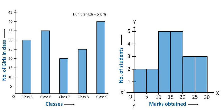
Compare frequency of continuous aata with equal bins
Use histograms to group continuous numerical data into adjacent intervals called bins, often of equal width. The height of each bar represents the frequency of data points in that bin, allowing easy comparison of how common different ranges of values are. For example, visualizing employee counts in different age ranges helps understand distribution briefly.
Analyze frequency with unequal bin widths
When bins vary in width, histogram bar height alone can be misleading. Instead, frequency density (frequency divided by bin width) determines bar height, so the area of each bar accurately reflects the count. This approach ensures correct interpretation of frequency when intervals are uneven.
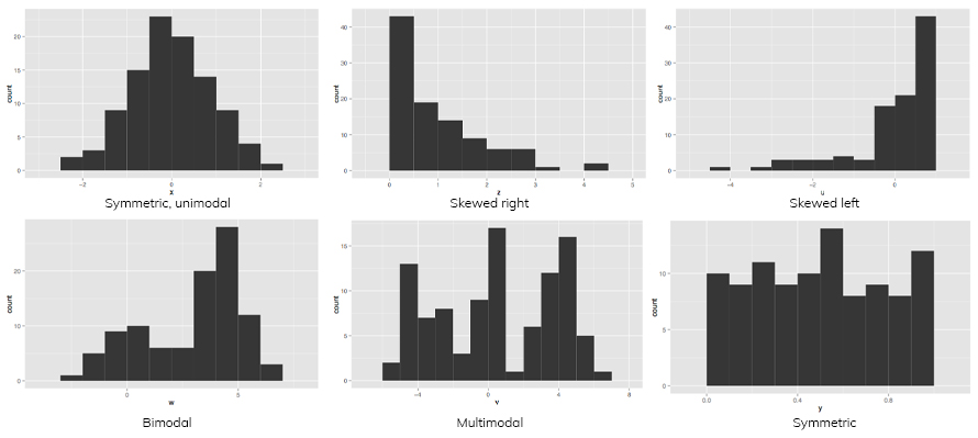
Identify statistical anomalies and distribution patterns
Histograms reveal data spread, outliers, and modes (peaks). They help detect if data clusters around one value (unimodal), two peaks (bimodal), or multiple peaks (multimodal), aiding diagnostics of data uniformity or underlying causes of anomalies.
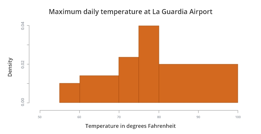
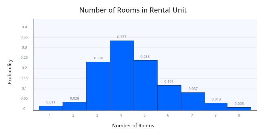
Visualize probability occurrences
Histograms provide a rough estimate of the probability distribution by showing how data values are concentrated. In density-based histograms, the total area normalizes to one, representing the probability density function.
Types of Histograms
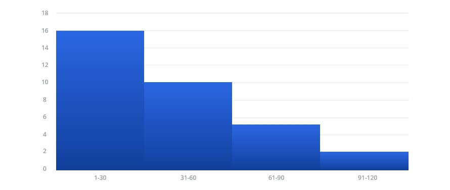
1. Equal Bin Width Histogram
This type groups data points into bins of equal size, with the height of each bar proportional to the frequency of data points in that bin. It’s the most common and straightforward histogram representation.
2. Variable Bin Width Histogram
When bins vary in size, the height of each bar represents frequency density (frequency divided by bin width), ensuring the area of the bar corresponds to the actual frequency. This allows accurate visualization even when bin sizes are unequal.
3. Normalized or Cumulative Histogram
A normalized histogram shows relative frequencies, where the sum of all bar heights equals 1, representing proportions instead of raw counts. Cumulative histograms display running totals, showing how frequencies accumulate across bins.
When Not to Use a Histogram?
For non-numerical or categorical data
Histograms are unsuitable for discrete or categorical variables. Instead, use bar charts, which clearly show gaps between bars to indicate distinct categories.
To show correlations between two variables
Histograms represent one variable’s distribution. For analyzing relationships or correlations between two variables, use scatter plots, line graphs, or other correlation charts.